bladeRF-car designed with DesignSpark Mechanical

BladeRF-car

A bladerf-car? Yes, somehow. In between my bladerf-project I played a lot with DesignSpark Mechanical, free 3D software.  And now in Holland there are fablabs. What is fablab? Fabrication-laboratory. A workshop with machines like 3D-printers and a laser cutter. Somewhere in the corner is a reprap busy reproducing itself… I am excited.

In the beginning of my career, before being a retired engineer, I was at the start of the computer age. My first job was maintenance of a PDP8 minicomputer. Later, many years later, there was my first PC with a 10 MB hard disk! 10 MB. Incredibly that an average hard disk now is at least 1TB, that is 1000 GB and 1 GB is 100 * 10 MB! So an average hard disk in a laptop (!) has a capacity of 100.000 times my first 10 MB hard disk. The same with memory, the same with transfer speed, the same with…

These times are incredible times. A few years ago I saw the first regular use of LEDs. Now I have a little pocket flashlight with an enormous amount of light. Ok, my old big maglite with 4 D-cells is still in my car if I need to impress someone. The 4 D-cells in an aluminium case impress more than the light of the small lamp inside that maglite however…

There is a new phenomenon: 3D printing. It is not new at all, but there is a breakthrough now. I feel that again I am at the start of something new, something that will change the world.

So, the last few weeks I was playing around with DesignSpark Mechanical. It is free 3D software. With it you can draw 3D objects and produce .STL files. Those files contain the info that a 3D printer needs to 3D print what you did draw with your 3D software. You can upload the file to a printer shop and some time later you get the stuff in real hardware in your postbox. Or you buy or build a 3D printer and print your creative work at home!

Have a look at http://www.thingiverse.com and see what others designed!

About 35 years ago I designed a car made from plywood. It was a kind of puzzle. But once you slide all the pieces in place you have a car to play with. I redesigned that same car with DesignSpark Mechanical. Just for fun and just because you can. I think I am gonna take a piece of Trespa and take it to the fablab. Then I might use a laser cutter to make this car into a real thing.

The car:

And a more or less exploded view:

How to put this all together?

First you take the left side (linkerzijde)

Now first take the bakdeksel (cover of the the rear area) and stick it in the left side:

Not take the right side (rechterzijde) and put it in place:

 Now is the time for the front plate (frontschot), you slide it upwards in place:

At last: the bottom plate (bodemplaat). This is a little tricky: you have to place it at the underside:

 of the car, push it upwards:

 and then slide it forwards. The result:

Or in the original perspective:

Now we can slide the window (voorruit) on its place:

And the roof (cabinedak) with result:

Finally the last two planes called tussenschot and achterschot:

As you can see these last two planes lock the bottom plate, and finally, there it is, the bladerf-car:

Some remarks:
• I designed the car from a plate with a thickness of 6 mm
• In DesignSpark Mechanical I named the various parts, so they can be separately designed
• I used mostly Select and Pull during the design
• It is very handy to select a surface and then choose Plan View to get a plane to draw upon
• With the pull tool you can remove parts by dragging backwards
• If you want to design something like this: study, do and perform all the tutorials and videos you can find on the Internet
it is really difficult at the start, but at the end you draw with ease and confidence!
• Use points, lines, rectangles and construction lines: you can delete them selectively when not needed anymore
• This car is a very simple example with flat planes, DesignSpark Mecanical can do a lot more!
• I did not laser cut or 3D-print this design. I expect some problems: perhaps the gaps should be wider, a fraction of a millimeter. And may be there are errors in this design…
• So, not any warranty, but don’t be afraid: do try this at home yourself!
• I am in no way involved with DesignSpark Mechanical, the software is free and I am just a happy old retired married satisfied customer, really!

The example above was an attempt to design something (the blue ring) to connect a circular LED light (the yellow thing) to the rectangular frame of a microscope (the orangish thing)
I wanted to 3D print the blue adapter but it proved to be a lot easier just to take a piece of plywood and a jigsaw…

Epilogue

At the end of the year, more than ever, I like to look back in (my) history. Because of my age there is more past than future! But the present is interesting enough, so I tend to stay in the present every day as long as I live. The last few weeks I was distracted from my dear bladerf-project because of DesignSpark Mechanical. I took that side path and enjoyed it a lot. I hope you enjoyed it too!
If you want the STL-files of the design of the bladerf-car: just send me an email and I will be more than happy to send it to you.

Happy Christmas, Happy New Year, Happy Whatever!

Que le vaya bien!

Without bladeRF: correlation with FFT and problem: python class returns by value

Python problem: class returns by reference, not by value

I made some changes to my python-class Gold.

The problem is that in python an attribute of a class is returned by reference. This might be nasty in some situations.

#import old class Gold goldutil
myGold1 = Gold(13)
prn = myGold1. prnRegAnalogue
prn[0] = 100
prn2 = myGold1. prnRegAnalogue

if I modify prn I modify the internal list prnRegAnalogue because they are identical: they have the same address!

So now prn[0] and prn2[0] both have the same value 100.

Therefore I changed my class. Now I hide prnRegAnalogue by prefixing the name with a double-underscore: __ prnRegAnalogue and I defined a method prnReg() to return a copy of prnRegAnalogue. The effect is that now the list prnRegAnalogue is called by value.

# import modified class Gold goldutil
myGold1 = Gold(13)
prn = myGold1. prnRegAnalogue
prn[0] = 100
prn2 = myGold1. prnRegAnalogue

Now prn2[0] has not been changed.

The new class now reads:

class Gold:
    
# Gold-sequence   goldutil.py
# Nov-2013 Kees de Groot
# call:
#   myprn1 = Gold(3, 7) for code phase selection = (3,7)
# or
#   myprn2 = Gold(4) for the 4th from the list
#    = satellite ID number = GPS PRN signal number

    # start with (0,0) to start numbering with 1
    # note that PRN 34 and 37 are identical
    prnlist = [ (0,0), (2,6), (3,7), (4,8), (5,9), (1,9),
                (2,10), (1,8), (2,9), (3,10), (2,3),
                (3,4), (5,6), (6,7), (7,8), (8,9),
                (9,10), (1,4), (2,5), (3,6), (4,7),
                (5,8), (6,9), (1,3), (4,6), (5,7),
                (6,8), (7,9), (8,10), (1,6), (2,7),
                (3,8), (4,9), (5,10), (4,10), (1,7),
                (2,8), (4,10)]

    def __init__(self, a, b = 0):
        self.reg1 = [1]*11         # don't use first bit-position [0]
        self.reg2 = [1]*11         # so count bit-positions from 1 to 10
        self.__prnRegBinary = []       # contains 0 and 1
        self.__prnRegAnalogue = []     # contains -1 and +1
        if b == 0:  # a = GPS PRN signal number or satellite ID
            (self.prn1, self.prn2) = self.prnlist[a]
        else:       # direct code phase selection
            (self.prn1, self.prn2) = (a, b)
        for i in range(1024):
            G1 = self.reg1[10]
            G2 = self.reg2[self.prn1] ^ self.reg2[self.prn2]
            out = G1 ^ G2
            self.__prnRegBinary.append(out)        # values 0 and 1
            self.__prnRegAnalogue.append(2*out-1)  # values -1 and +1
            val1 = self.reg1[3] ^ self.reg1[10]
            val2 = (self.reg2[2] ^ self.reg2[3] ^ self.reg2[6] ^
                    self.reg2[8] ^ self.reg2[9] ^ self.reg2[10])
            # shift one position to the right
            for j in range(9):  # j = 0,1,2,3,4,5,6,7,8
                k = 10 - j      # k = 10,9,8,7,6,5,4,3,2
                self.reg1[k] = self.reg1[k-1]
                self.reg2[k] = self.reg2[k-1]
            self.reg1[1] = val1
            self.reg2[1] = val2

    # return list by value, not by reference
    def prnReg(self):
        alist = []
        for val in self.__prnRegAnalogue:
            alist.append(val)
        return alist

Correlation with fft

A very interesting property of the Fourier transform is that convolution in the time-domain can be done by multiplication in the frequency-domain.
That means that to calculate a @ b, in which @ is meant to stand for convolution, you can do that calculation as follows:

ifft( fft(a) * fft(b) )

which means do an fft of a, do an fft of b, multiply and inverse-fft the result.
But the result of fft(a) has to be complex conjugated first, which means that all imaginary values has to change sign.
So, the procedure is: ifft(conjugate(fft(a)) * fft(b))
It sound strange perhaps, but this complex (sic) procedure might be very efficient to calculate because in practice the part conjugate(fft(a)) has to be calculated only once during initialization. The remaining calculation boils down to
c = conjugate(fft(a)
…
ifft(c * fft(b))

To calculate the correlation between a and b.

I made a small python program to experiment with this procedure:

import goldutil as gl   # home-made Gold-sequence generator
import pylab as pl      # module for plotting
import numpy as np      # module for fft

# CorrelFFTdemo2s.py
# Simulation of message constructed using Gold-sequences
# - Define an 8-bit message: eg 0 0 1 1 0 1 0 0 1 = -1, 1, 1, -1, 1, -1, -1, 1
# - Construct an array with 9*1024 samples of the same Gold-sequence,
#      eg. satellite id 12
# - Multiply the first 1024 samples with 1, the 2n set with -1,
#      the 3rd set with -1, etc to code our message
# - Now try to decode our message using correlation implemented with FFT
# nov 2013 Kees de Groot

messageBin = (0, 0, 1, 1, 0, 1, 0, 0, 1)
print "messageBin = ", messageBin
messageAna = []
for val in messageBin:
    messageAna.append(2*val-1)
print "messageAna = ", messageAna

sat1 = 12                   # this is the sat we are looking for
myGold1 = gl.Gold(sat1)
pprn1 = myGold1.prnReg()    # get list with 1024 bits of Goldsequence

# code message into codedmsg by multiplying
codedmsg = []
for mesbit in messageAna:
    for prnbit in pprn1:
        codedmsg.append(mesbit * prnbit)
codedmsg = [0]*200 + codedmsg # add some zeroes to improve readability of plot

# decode codedmsg by correlation with origional pprn1 Gold-sequence

# cross-correlation with the right Gold-sequence
# correlate codedmsg with pprn1 and put result in ac

# once-only calculate complex conjugate of prn-sequence pprn1
# problem is that I want the fft to have the same length as codedmsg
# so, just add zeros at the end of pprn1

numzeros = len(codedmsg) - len(pprn1)
pprn1 = pprn1 + [0]*numzeros

fftprn =  np.fft.rfft(pprn1)
# complex conjugate (there must be a better method)
for i in range(len(fftprn)):
    fftprn[i] = fftprn[i].conjugate()

fftcodedmsg = np.fft.rfft(codedmsg)

# convolution (correlation) == multiplying with complex conjugate
#           after fft and inverse-fft the result

# multiply fftcodedmsg with fftprn
for i in range(len(fftcodedmsg)):
    fftcodedmsg[i] *= fftprn[i]
# inverse-fft
ac = np.fft.irfft(fftcodedmsg)

pl.figure(1)
pl.title("correlation, calculated with fft-method")
pl.ylim(-1500, 1500)
pl.stem(ac)
pl.show()

This program might look daunting, but there is really a lot of comment and not so much code.

The output is:

Python 2.7.3 (default, Apr 10 2012, 23:31:26) [MSC v.1500 32 bit (Intel)] on win32
Type "copyright", "credits" or "license()" for more information.
>>> ================================ RESTART ================================
>>> 
messageBin =  (0, 0, 1, 1, 0, 1, 0, 0, 1)
messageAna =  [-1, -1, 1, 1, -1, 1, -1, -1, 1]

Graphics

It is obvious that this is exactly the same result as in the previous blog-message where I programmed plain convolution.

Correlation with fft, block-mode

I expect to handle my real-time samples in blocks of 1024 chips. A chip is one bit of a Gold-sequence. In this example I simulated this procedure. In a loop I correlate 1024 chips from my input and decode the message bit by bit.

import goldutil as gl   # home-made Gold-sequence generator
import pylab as pl      # module for plotting
import numpy as np      # module for fft

# CorrelFFTblock.py
# Simulation of message constructed using Gold-sequences
# - Define an 8-bit message: eg 0 0 1 1 0 1 0 0 1 = -1, 1, 1, -1, 1, -1, -1, 1
# - Construct an array with 9*1024 samples of the same Gold-sequence,
#      eg. satellite id 12
# - Multiply the first 1024 samples with 1, the 2n set with -1,
#      the 3rd set with -1, etc to code our message
# - Now try to decode our message using correlation implemented with FFT
# do this piece-wise in blocks of 1024 bits
# nov 2013 Kees de Groot

def minmax(ac):
    minval = min(ac)
    maxval = max(ac)
    if abs(minval) > abs(maxval):
        result = 0
    else:
        result = 1
    return result

messageBin = (0, 0, 1, 1, 0, 1, 0, 0, 1)
print "messageBin = ", messageBin
messageAna = []
for val in messageBin:
    messageAna.append(2*val-1)
print "messageAna = ", messageAna

sat1 = 12                   # this is the sat we are looking for
myGold1 = gl.Gold(sat1)
pprn1 = myGold1.prnReg()    # get list with 1024 bits of Goldsequence

# code message into codedmsg by multiplying
codedmsg = []
for mesbit in messageAna:
    for prnbit in pprn1:
        codedmsg.append(mesbit * prnbit)
codedmsg = [0]*200 + codedmsg + [0]*824 # add some zeroes

# decode codedmsg by correlation with origional pprn1 Gold-sequence

# cross-correlation with the right Gold-sequence
# correlate codedmsg with pprn1 and put result in ac
# once-only calculate complex conjugate of prn-sequence pprn1

fftprn =  np.fft.rfft(pprn1)
# complex conjugate (there must be a better method)
for i in range(len(fftprn)):
    fftprn[i] = fftprn[i].conjugate()

# the above calculation has to be done once during initialization
# now take 1024 bit blocks and correlate using fft

N = len(codedmsg) / len(pprn1)
print "N = ", N

for n in range(N):
    fftcodedmsg = np.fft.rfft(codedmsg[n*1024:(n+1)*1024])
    for i in range(len(fftcodedmsg)):
        fftcodedmsg[i] *= fftprn[i]
    ac = np.fft.irfft(fftcodedmsg)
    print "block ", n, ", message-bit = ", minmax(ac)
    pl.figure(n+1)
    pl.title("correlation, calculated with fft-method " + "block " + str(n))
    pl.ylim(-1500, 1500)
    pl.stem(ac)

pl.show()

with output:

Python 2.7.3 (default, Apr 10 2012, 23:31:26) [MSC v.1500 32 bit (Intel)] on win32
Type "copyright", "credits" or "license()" for more information.
>>> ================================ RESTART ================================
>>> 
messageBin =  (0, 0, 1, 1, 0, 1, 0, 0, 1)
messageAna =  [-1, -1, 1, 1, -1, 1, -1, -1, 1]
N =  10
block  0 , message-bit =  0
block  1 , message-bit =  0
block  2 , message-bit =  1
block  3 , message-bit =  1
block  4 , message-bit =  0
block  5 , message-bit =  1
block  6 , message-bit =  0
block  7 , message-bit =  0
block  8 , message-bit =  1
block  9 , message-bit =  1

and a lot of nice graphics:

Conclusion

To find a message coded with a Gold-sequence one uses correlation. One method is to use convolution. It is a simple process but might cost a lot of time.

Another method is to make use of a property of the Fourier-transform:

Convolution in the time-domain is the same as multiplication in the frequency-domain

I experimented with this method and showed it to be possible.
Now I am confident to use this method with real samples from the bladeRF.

Keep tuned!

For GPS on a bladeRF you have to start with Gold-sequences to find signals buried in noise: it is all about correlation

Gold-sequence

GPS-signals is all about correlation. The signals are completely buried in the noise. Only by searching (or knowing) the code-sequences and the Doppler frequencies is it possible to decode the signals. And they are all transmitted at that same frequency!

I did some experiments in python to get aquainted (again) with Gold-sequences and correlation. So, I programmed a class Gold and wrote some test-programs. Very nice experiments!

I had a lot of fun with it. Python is a very simple language. Plotting is a breeze. And with a class that you can import you get nice short programs. The IDLE editor is sufficient to get experiments running.


A very nice article is: “Understanding Spread Spectrum for Communications” at http://www.ni.com/white-paper/4450/en/

A python class "Gold"

In python I programmed the following class:

class Gold:
    
# Gold-sequence   goldutil.py
# Nov-2013 Kees de Groot
# call:
#   myprn1 = Gold(3, 7) for code phase selection = (3,7)
# or
#   myprn2 = Gold(4) for the 4th from the list
#    = satellite ID number = GPS PRN signal number

    # start with (0,0) to start numbering with 1
    # note that PRN 34 and 37 are identical
    prnlist = [ (0,0), (2,6), (3,7), (4,8), (5,9), (1,9),
                (2,10), (1,8), (2,9), (3,10), (2,3),
                (3,4), (5,6), (6,7), (7,8), (8,9),
                (9,10), (1,4), (2,5), (3,6), (4,7),
                (5,8), (6,9), (1,3), (4,6), (5,7),
                (6,8), (7,9), (8,10), (1,6), (2,7),
                (3,8), (4,9), (5,10), (4,10), (1,7),
                (2,8), (4,10)]


    def __init__(self, a, b = 0):
        self.shreg1 = [1]*11         # don't use first bit-position [0]
        self.shreg2 = [1]*11         # so count bit-positions from 1 to 10
        self.prnRegBinary = []       # contains 0 and 1
        self.prnRegAnalogue = []     # contains -1 and +1
        if b == 0:  # a = GPS PRN signal number or satellite ID
            (self.prn1, self.prn2) = self.prnlist[a]
        else:       # direct code phase selection
            (self.prn1, self.prn2) = (a, b)
        for i in range(1024):
            G1 = self.shreg1[10]
            G2 = self.shreg2[self.prn1] ^ self.shreg2[self.prn2]
            out = G1 ^ G2
            self.prnRegBinary.append(out)
            self.prnRegAnalogue.append(2*out-1)
            val1 = self.shreg1[3] ^ self.shreg1[10]
            val2 = (self.shreg2[2] ^ self.shreg2[3] ^ self.shreg2[6] ^
                    self.shreg2[8] ^ self.shreg2[9] ^ self.shreg2[10])
            # shift one position to the left
            for j in range(9):
                k = 10 - j
                self.shreg1[k] = self.shreg1[k-1]
                self.shreg2[k] = self.shreg2[k-1]
            self.shreg1[1] = val1
            self.shreg2[1] = val2

A first test-program:

import goldutil as gl

myGold37 = gl.Gold(3, 7)
prn1 = myGold37.prnRegBinary
prn2 = myGold37.prnRegAnalogue

print "the first 20 points of the binary version of Gold37:"
for i in range(20):
    print prn1[i],
print "\n..."
print "\nthe first 20 points of the analogue version of Gold37:"
for i in range(20):
    print prn2[i],
print "\n..."

with output:

Python 2.7.3 (default, Apr 10 2012, 23:31:26) [MSC v.1500 32 bit (Intel)] on win32
Type "copyright", "credits" or "license()" for more information.
>>> ================================ RESTART ================================
>>> 
the first 20 points of the binary version of Gold37:
1 1 1 0 0 1 0 0 0 0 1 1 1 0 0 0 0 0 1 1 
...

the first 20 points of the analogue version of Gold37:
1 1 1 -1 -1 1 -1 -1 -1 -1 1 1 1 -1 -1 -1 -1 -1 1 1 
...
>>>

With this framework I can write simple programs by importing the class Gold with the command
import goldutil as gl

Autocorrelation

As a first test I calculate autocorrelation.

# Gold02b.py
# autocorrelation
# nov-2013 Kees de Groot

import goldutil as gl
import pylab as pl

myGold37 = gl.Gold(3, 7)
prn2 = myGold37.prnRegAnalogue

# autocorrelation
ac = [0]*1024
for m in range(1024):
    for l in range(1024):
        ac[m] += prn2[l] * prn2[(l + m)%1024]
print "\nthe first 20 points of the autocorrelation of myGold37:"
for i in range(20):
    print ac[i],
print "\n..."
pl.figure(1)
pl.title("autocorrelation, note big peak of 1024 at x = 0")
pl.vlines(range(1024),[0]*1024,ac)
pl.show()

with output:

Python 2.7.3 (default, Apr 10 2012, 23:31:26) [MSC v.1500 32 bit (Intel)] on win32
Type "copyright", "credits" or "license()" for more information.
>>> ================================ RESTART ================================
>>> 

the first 20 points of the autocorrelation of myGold37:
1024 0 0 0 -68 -4 0 0 60 -8 4 4 -4 0 -4 60 64 60 -8 4 
...

There is nice peak at x=0, indicating positive correlation, the codes overlaps perfectly

Now correlate two different Gold-sequences.

# Gold02c.py
# correlation between different Gold-sequences
# nov-2013 Kees de Groot

import goldutil as gl
import pylab as pl

myGold37 = gl.Gold(3, 7)       # code (3,7)
prn1 = myGold37.prnRegAnalogue
myGold15 = gl.Gold(15)         # satellite 15
prn2 = myGold15.prnRegAnalogue

# correlation

ac = [0]*1024
for m in range(1024):
    for l in range(1024):
        ac[m] += prn1[l] * prn2[(l + m)%1024]
print "\nthe first 20 points of the correlation:"
for i in range(20):
    print ac[i],
print "\n..."
pl.figure(1)
pl.title("correlation between two different Gold-codes")
pl.vlines(range(1024),[0]*1024,ac)
pl.show()

with output:

Python 2.7.3 (default, Apr 10 2012, 23:31:26) [MSC v.1500 32 bit (Intel)] on win32
Type "copyright", "credits" or "license()" for more information.
>>> ================================ RESTART ================================
>>> 

the first 20 points of the correlation:
0 0 0 -64 0 0 0 0 0 -4 64 0 4 -4 -64 0 -4 -68 0 64 
...

There are some peaks, but not a single strong one, so there is no correlation.

The real thing

Now it is time for the real thing.

• Take a Gold-sequence of sat 18
• Shift it to the right 200 chips
• Add two more Gold-sequences: sat 4 and sat 17
• Now I have a shifted contaminated satellite signal.

First correlate with a Gold-sequence sat=20. Of course there is not any correlation, only noise
Then, the wonder: correlate with a Gold-sequence sat=18. We see an obvious peak at x=200.
So we know we found the satellite and we know the delay of the signal!

import goldutil1 as gl
import pylab as pl

# Gold04.py
# Generate a Gold-sequence, shift it 200 chips
#       and add two more different Gold-sequences
# then, correlate it with an arbitrary Gold-sequence
# and finally correlate it with the same Gold-sequence
# nov 2013 Kees de Groot

sat1 = 18                       # this is the sat we are looking for
myGold1 = gl.Gold(sat1)
pprn1 = myGold1.prnRegAnalogue

sat2 = 20                       # this is our guess1
myGold2a = gl.Gold(sat2)
pprn2a = myGold2a.prnRegAnalogue

sat2 = 18                       # this is our guess2
myGold2b = gl.Gold(sat2)
pprn2b = myGold2b.prnRegAnalogue

# shift pprn1 200 bits to the right
k = 200
for i in range(1024):
    temp = pprn1[(i + k)%1024]
    pprn1[(i + k)%1024] = pprn1[i]
    pprn1[i] = temp

# add two different Gold-sequences to pprn1
myGold3 = gl.Gold(4)
myGold4 = gl.Gold(17)
for i in range(1024):
    pprn1[i] = (pprn1[i] + myGold3.prnRegAnalogue[i] +
                myGold4.prnRegAnalogue[i])

# now pprn1 is contaminated with two other sequences
    
# cross-correlation with wrong Gold-sequence
ac = [0]*1024
for m in range(1024):
    for l in range(1024):
        ac[m] += pprn1[l] * pprn2a[(l + m)%1024]
print "\n 20 points around the peak at 200:"
for i in range(190, 210):
    print ac[i],
print "\n..."
pl.figure(1)
pl.title("correlation with different sequence")
pl.vlines(range(1024),[0]*1024,ac)

# cross-correlation with the right Gold-sequence
ac = [0]*1024
for m in range(1024):
    for l in range(1024):
        ac[m] += pprn1[l] * pprn2b[(l + m)%1024]
print "\n 20 points around the peak at 200:"
for i in range(190, 210):
    print ac[i],
print "\n..."
pl.figure(2)
pl.title("correlation with the right sequence")
pl.vlines(range(1024),[0]*1024,ac)

pl.show()

With output:

Python 2.7.3 (default, Apr 10 2012, 23:31:26) [MSC v.1500 32 bit (Intel)] on win32
Type "copyright", "credits" or "license()" for more information.
>>> ================================ RESTART ================================
>>> 

 20 points around the peak at 200:
12 116 112 28 4 -4 -8 12 0 -48 -48 -36 -8 128 8 -4 -88 -20 -24 -28 
...

 20 points around the peak at 200:
48 104 124 184 72 -12 -32 0 60 8 708 -40 -20 -32 -32 80 12 -24 -80 -48 
...

Note there is no peak in the first run, but in the second run there is a peak with a value of 708, indicating strong correlation around delay = 200 chips.

Only noisy correlation, not one obvious peak

And there it is: a peak around x=200. A clear indication of the existence of a signal in the noise.

Conclusion:

I implemented the Gold-sequence as a class Gold in python.
With that class I first demonstrated a working implementation.
Then I did some experiments with (auto)correlation and finally demonstrated that you can find a certain code-sequence in a noisy contaminated signal and even calculate the delay of that signal.

BladeRF data around GPS frequency of 1575.42 MHz

GPS revisited and some confessions

The book

An interesting book is:

 "A software defined GPS and Galileo receiver" , a single frequency approach, by Kai Borre et al.

In the back of the book is a CDROM with a dataset. That dataset contains the if-output of a real SDR tuned to a GPS-signal. I copied the test-file to a convenient place and renamed it to testdata.dat.

That started my struggle with GPS. In that timeperiod I did a course on java and wanted to do something ‘useful’ with that knowledge. I decided to build a GPS-receiver and program it in java. So, I bought some books, read a lot about it on the internet and really got a deep understanding of the system and the signals used in a GNSS-system.

I decided to first develop the software and later concentrate on the hardware. The software was difficult enough for me…

To make a really long story short I finally managed to read almanac-data from the GPS-signals. However I got stuck in the tracking loop. I never got the loop stable. That last problem never made it to my blog at http://www.qsl.net/pa1kdg/ by the way.

So, I also did not succeed in calculating the position from the data in that huge data-file. But, what the heck, I learned soo much of that whole project…

Next step

My next step now is restart that whole project with a bladeRF-board. I want to use python now as a programming language. Just because I can ;>))

TANSTAAFL There aint no such thing as a free lunch

Being a retired engineer, the Mathworks, the developers of MATLAB, is no longer interested in me. When I worked at Wageningen University and Research I got an enormous lot of software free. I was addicted to MATLAB (and LABVIEW by the way), with that software you can solve all your scientific problems. After my retirement I soon discovered that the love of the Mathworks I felt was quite different than real life love I perceive on a daily basis from the people around me. Just before retirement I got an SDR-board with a huge Xilinx FPGA. That would be my big and only project after retirement! Nope, Xilinx too discovered I am not longer interesting for them. Real-life for a CEO is about earning money, not about supporting retired engineers. I have not any problem to pay for hardware or software but 2000 bucks for my hobby is in-explainable to my wife (ok, this whole hobby is inexplainable…) OK, I am back on earth now with two feet on the ground, with my bladeRF and open source software. This is my real life now!!

Life is complicated though

On my way along my GPS-project I discovered a lot about linux, VMWare, github, python-eggs, C, VHDL, makefiles, Quartus, SDR-Radio, gnuradio, Octavo and finally plotting in python (and kind of python-MATLAB too). And I found many sidepaths, DesignSpark Mechanical e.g. and soldering SMD’s.

What now

Back to GPS. I want to record a data-file with real-bladeRF-data and try to process that file. First discover what satellites are visible, later read the almanac data. Finally try to get past that data-tracking-loop problem and solve the position-equations. In the meantime I want to try to get some calculations done in the FPGA. It should be possible to do the correlation-part in the FPGA. Quite a challenge!

Some facts

I concentrate on GPS, not GLONASS. GPS transmits on one frequency. All satellites transmit on the same frequency, that is to say, because of Doppler effects there is a slight deviation of that frequency for every satellite. Each satellite has a different code. If you know the code and the Doppler-frequency you can decode the signal of that very satellite. The signal is simply almanac-data at 50 baud. The satellites tell you constantly where they are. Because you know exactly which bit of the code-sequence you receive and because you ‘see’ 4 satelites or more you can calculate where your GPS-antenna is. For 50 $ you can buy a module that does this trick in a very good way, so…

Practical now

Ok, I tune bladeRF to 1575.42 MHz. With a bandwidth of 2 MHz I might expect to get a weak noisy signal, barely a signal, -160dBW. So, only noise.

There are 32 different code sequences. Just try all those sequences one by one.

There are about 60 different frequencies to consider because of the unknown Doppler shift. So try all frequencies.

In a 3D-display one can find some peaks. Then you know some codes and some Doppler shifts. From then on you can decode the satellite signals and get the almanac data. Then you know te distance to each found satellite. In 3D, if you know the distance to 3 or more satellites, you can calculate where you are.  Because you know where the satellites are you know where you are. Simple eh? That is GPS

GLONASS, the Russian system, uses different frequencies. No problem, bladeRF can handle that too. And, with an FPGA you can put the most time-consuming calculations on that chip.

That is the theory.

Tune to 1575.42 MHz. Bandwidth 2 MHz, so samplerate 4 MHz. VGA-gains at 30 dB. Get 1M samples into a file. Perform an FFT. Hopefully something interesting will show up.

Filename A1575.csv without GPSantenna connected and B1575.csv with the GPSantenna connected and pearing out of my window. In the meantime I have a TomTom and a Garmin device locked at the satellites in the sky so I know some data already.

Got my first two files with bladeRF-cli. GPS-systems say: satellites in the sky: 2,4,5,8,9,10,13,16 of which 2,4, 9 are strongest. So I might see satellites 2, 4 and 9 in my datafiles.

[INFO] Using libusb version 1.0.16.10774
[INFO] Found a bladeRF
[INFO] Claimed all inferfaces successfully
[WARNING] extract_field: Field checksum mismatch
[WARNING] Could not extract VCTCXO trim value
[WARNING] extract_field: Field checksum mismatch
[WARNING] Could not extract FPGA size
bladeRF> load fpga hostedx115.rbf
Loading fpga from hostedx115.rbf...
[INFO] Change to alternate interface 3
[INFO] Change to alternate interface 1
[INFO] Changed into RF link mode: LIBUSB_SUCCESS / LIBUSB_TRANSFER_COMPLETED
[INFO] Setting integer sample rate: 1000000
[INFO] Found r value of: 4
[INFO] MSx a + b/c: 316 + 4/5
[INFO] MSx a + b/c: 316 + 4/5
[INFO] MSx P1: 0x00009c66 (40038) P2: 0x00000002 (2) P3: 0x00000005 (5)
[INFO] Calculated samplerate: 1000000 + 0/1
[INFO] Set actual integer sample rate: 1000000
[INFO] Setting integer sample rate: 1000000
[INFO] Found r value of: 4
[INFO] MSx a + b/c: 316 + 4/5
[INFO] MSx a + b/c: 316 + 4/5
[INFO] MSx P1: 0x00009c66 (40038) P2: 0x00000002 (2) P3: 0x00000005 (5)
[INFO] Calculated samplerate: 1000000 + 0/1
[INFO] Set actual integer sample rate: 1000000
Done.
bladeRF> print rxvga1

  RXVGA1 Gain:  33

bladeRF> print rxvga2

  RXVGA2 Gain:   3dB

bladeRF> set rxvga2 33
[WARNING] Setting gain above 30dB? You crazy!!
bladeRF> set rxvga2 30
bladeRF> print rxvga2

  RXVGA2 Gain:  30dB

bladeRF> set bandwidth 2000000

  Set RX bandwidth - req:  2000000Hz actual:  2500000Hz
  Set TX bandwidth - req:  2000000Hz actual:  2500000Hz

bladeRF> set frequency 1575420000

  Set RX frequency: 1575420000Hz
  Set TX frequency: 1575420000Hz

bladeRF> set bandwidth 2000000

  Set RX bandwidth - req:  2000000Hz actual:  2500000Hz
  Set TX bandwidth - req:  2000000Hz actual:  2500000Hz

bladeRF> set samplerate 4000000

[INFO] Setting integer sample rate: 4000000
[INFO] Found r value of: 1
[INFO] MSx a + b/c: 316 + 4/5
[INFO] MSx a + b/c: 316 + 4/5
[INFO] MSx P1: 0x00009c66 (40038) P2: 0x00000002 (2) P3: 0x00000005 (5)
[INFO] Calculated samplerate: 4000000 + 0/1
[INFO] Set actual integer sample rate: 4000000
  Setting RX sample rate - req:   4000000Hz, actual:   4000000Hz
[INFO] Setting integer sample rate: 4000000
[INFO] Found r value of: 1
[INFO] MSx a + b/c: 316 + 4/5
[INFO] MSx a + b/c: 316 + 4/5
[INFO] MSx P1: 0x00009c66 (40038) P2: 0x00000002 (2) P3: 0x00000005 (5)
[INFO] Calculated samplerate: 4000000 + 0/1
[INFO] Set actual integer sample rate: 4000000
  Setting TX sample rate - req:   4000000Hz, actual:   4000000Hz

bladeRF> set bandwidth 2000000

  Set RX bandwidth - req:  2000000Hz actual:  2500000Hz
  Set TX bandwidth - req:  2000000Hz actual:  2500000Hz

bladeRF> rx config format=csv n=1000000 file=/temp/A1575.csv
bladeRF> rx start
bladeRF> rx start
bladeRF> rx start
bladeRF> rx config format=csv n=1000000 file=/temp/B1575.csv
bladeRF> rx start
bladeRF> rx start
bladeRF> rx start
bladeRF>

Note the warning about gain higher than 30 dB ;>))

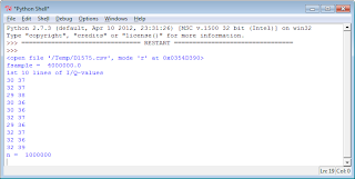
# FFTSDRdata03.py
# Nov-2013 Kees de Groot
#
# show and analyse snapshot file from bladeRF
# remove DC-component
# show data in different ways; I/Q, realtimeplot, FFT

import pylab as pl
import numpy as np
import math

filename = 'B1575.csv'
fsample = 4E6
timestep = 1 / fsample

f = open('/Temp/' + filename, 'r')
print f
print "fsample = ", fsample

dataI = []
dataQ = []

n = 0
sumI = 0
sumQ = 0
# read I, Q - values into memory
for line in f:
    list = line.split(',') # two values with comma inbetween
    Q = int(list[0])
    I = int(list[1])
    # print 1st 10 lines of data-file
    if n == 0:
        print '1st 10 lines of I/Q-values'
    if n < 10:
        print I, Q
    dataI.append(I) # save data in memory
    dataQ.append(Q)    
    sumI += I
    sumQ += Q
    n += 1
    
averI = sumI / n  # calculate average
averQ = sumQ / n

#averI = 0 # debug
#averQ = 0 # debug

print "n = ", n

# remove DC-component and construct complex dataC
dataC = []
for i in range(n):
    I = dataI[i] - averI
    Q = dataQ[i] - averQ
    dataI[i] = I
    dataQ[i] = Q
    dataC.append(complex(I,Q))  # this one has complex data
    
pl.figure(1)
pl.title("Q versus I of " + filename)
pl.xlabel('=======>  I')
pl.ylabel('=======>  Q')
pl.plot(dataI, dataQ, 'ro')

pl.figure(2)
pl.subplot(211)
pl.title("I-values of " + filename)
pl.ylabel('=======>  I')
pl.plot(dataI)
pl.subplot(212)
pl.title("Q-values of " + filename)
pl.ylabel('=======>  Q')
pl.plot(dataQ)

pl.figure(3)
sp = np.fft.fft(dataC)      # use fft, not rfft, since dataC is complex
freq = np.fft.fftfreq(n, d=timestep)    # for convenient x-axis-ticks
pl.title('fft of ' + filename)
pl.xlabel('frequency')
pl.ylabel('magnitude')
pl.plot(freq, abs(sp)/n)    # abs converts to magnitude; /n normalizes 

pl.show()

Run the program for the file without antenna connected: I would expect simply noise but there are three peaks at -583kHz, 0 kHz and 1022 kHz. Perhaps the gain was too big

I would expect simply noise but there are three peaks at
-583kHz, 0 kHz and 1022 kHz.

Now connect GPS-antenna

Perhaps the gain was too big

bladeRF> set rxvga2 27
bladeRF> set rxvga1 27
bladeRF> rx config format=csv n=1000000 file=/temp/C1575.csv
bladeRF> rx start
bladeRF> rx start
bladeRF> rx start
bladeRF>

I am still puzzled about the fact that I see a signal when no antenna is connected. I remove the SMB cable from RX and set gains to 0 dB. Then create file D1575.csv:

Biggest peak is at 0 Hz exactly, the other is at 1.01882E6, so around 1 MHz

Again without antenna but a 50 ohm dummyload directly connected to bladeRF-RX-input.
Something went wrong with the board. Error because of physical touching it with too big dummyload directly connected?

[INFO] Using libusb version 1.0.16.10774
[INFO] Found a bladeRF
[INFO] Claimed all inferfaces successfully
[WARNING] extract_field: Field checksum mismatch
[WARNING] Could not extract VCTCXO trim value
[WARNING] extract_field: Field checksum mismatch
[WARNING] Could not extract FPGA size
bladeRF> load fpga hostedx115.rbf
Loading fpga from hostedx115.rbf...
[INFO] Change to alternate interface 3
[INFO] Change to alternate interface 1
[INFO] Changed into RF link mode: LIBUSB_SUCCESS / LIBUSB_TRANSFER_COMPLETED
[INFO] Setting integer sample rate: 1000000
[INFO] Found r value of: 4
[INFO] MSx a + b/c: 316 + 4/5
[INFO] MSx a + b/c: 316 + 4/5
[INFO] MSx P1: 0x00009c66 (40038) P2: 0x00000002 (2) P3: 0x00000005 (5)
[INFO] Calculated samplerate: 1000000 + 0/1
[INFO] Set actual integer sample rate: 1000000
[INFO] Setting integer sample rate: 1000000
[INFO] Found r value of: 4
[INFO] MSx a + b/c: 316 + 4/5
[INFO] MSx a + b/c: 316 + 4/5
[INFO] MSx P1: 0x00009c66 (40038) P2: 0x00000002 (2) P3: 0x00000005 (5)
[INFO] Calculated samplerate: 1000000 + 0/1
[INFO] Set actual integer sample rate: 1000000
Done.
bladeRF> print rxvga1

  RXVGA1 Gain:  33

bladeRF> set rxvga1 0
bladeRF> set rxvga2 0
bladeRF> set samplerate 1000000

[INFO] Setting integer sample rate: 1000000
[INFO] Found r value of: 4
[INFO] MSx a + b/c: 316 + 4/5
[INFO] MSx a + b/c: 316 + 4/5
[INFO] MSx P1: 0x00009c66 (40038) P2: 0x00000002 (2) P3: 0x00000005 (5)
[INFO] Calculated samplerate: 1000000 + 0/1
[INFO] Set actual integer sample rate: 1000000
  Setting RX sample rate - req:   1000000Hz, actual:   1000000Hz
[INFO] Setting integer sample rate: 1000000
[INFO] Found r value of: 4
[INFO] MSx a + b/c: 316 + 4/5
[INFO] MSx a + b/c: 316 + 4/5
[INFO] MSx P1: 0x00009c66 (40038) P2: 0x00000002 (2) P3: 0x00000005 (5)
[INFO] Calculated samplerate: 1000000 + 0/1
[INFO] Set actual integer sample rate: 1000000
  Setting TX sample rate - req:   1000000Hz, actual:   1000000Hz

bladeRF> set frequency 1575420000

  Set RX frequency: 1575420000Hz
  Set TX frequency: 1575420000Hz

bladeRF> set bandwidth 2000000

  Set RX bandwidth - req:  2000000Hz actual:  2500000Hz
  Set TX bandwidth - req:  2000000Hz actual:  2500000Hz

bladeRF> rx config format=csv n=1000000 file=/temp/E1575.csv
bladeRF> start

Unrecognized command: start

bladeRF> rx start
bladeRF> rx start

Error: Operation invalid in current state

bladeRF> rx start
bladeRF> rx start
bladeRF> rx start
bladeRF>

Beware: sample rate = 1 Mhz

One peak at zero Hz, the other is at 19.354 Hz.
Now samplerate = 2 MHz

Now same with samplerate = 4MHz

Still, no antenna connected, but dummyload directly at RX

Conclusion

I have a problem. I expected a flat noise floor without any antenna connected. But I see some spurious signals. I might be able to explain the signal at 0 Hz. But the others are strange.

I have to check again without any antenna connected and vary the parameters that I can set:

n, the number of samples, it might be a hickup of the interface

samplerate, there is a clock, so there are some signals

frequency, mixer-products?

rxvga1 the more gain, the more spurious signals

rxvga2 same

bandwidth, dont think so

Well I had a nice evening trying to get a GPS-satellite-signal but discovered my bladeRF also is very creative?